Python & Numerical Computing · Sep 2026 · 13 min read

A Monte Carlo Option Pricer, Checked Against the Closed Form

European option pricing via Monte Carlo simulation of GBM, validated against Black-Scholes — real spot price, real historical volatility, and a measured convergence curve instead of an asserted one.

Checking a Simulation Against the Answer You Already Know

Most of the numerical-Python work in this portfolio is FinOps pipelines and cloud cost data — this one is different: a Monte Carlo European option pricer, checked against the closed-form Black-Scholes price it should converge to. The reason to build this alongside FinOps work isn't a pivot into derivatives trading; it's the same underlying skill — numerical simulation, variance reduction, and being honest about what a model's confidence interval actually claims — applied to a problem that happens to have an exact answer to check against, which makes correctness bugs impossible to hide.

Live repo: monte-carlo-option-pricer

Before Step 1, one term this walkthrough leans on:

Antithetic variates — a variance-reduction technique: for every random draw Z used to simulate a price path, also simulate the path using -Z. The two paths are negatively correlated, which shrinks the variance of their averaged payoff below what the same number of independent draws would give — a real, measurable reduction in standard error, not a heuristic.

Step 1 — Ground the inputs in a real ticker, not invented numbers

def fetch_spot_and_realized_vol(ticker: str, lookback_days: int = 252) -> dict:
    hist = yf.Ticker(ticker).history(period="1y")
    closes = hist["Close"].tail(lookback_days + 1)
    log_returns = np.log(closes / closes.shift(1)).dropna()

    spot = float(closes.iloc[-1])
    annualized_vol = float(log_returns.std() * np.sqrt(252))
    return {"spot": spot, "annualized_realized_vol": annualized_vol, ...}

Running this against AAPL on 2026-09-17: a real spot price of $335.63, and a real annualized realized volatility of 0.2509 computed from 251 actual trading days of log returns — not a textbook sigma = 0.2 picked because it's round.

The honest limitation worth stating up front: this is realized (backward-looking, historical) volatility, not implied volatility from a live options-chain feed. Real implied vol needs a paid market-data source this project doesn't have. Realized vol is a standard, defensible substitute for illustration — it is not a claim that this matches what the option would actually trade at on an exchange today.

Step 2 — Simulate terminal prices under GBM, with antithetic variates

def simulate_terminal_prices(S0, r, sigma, T, n_paths, seed=None, antithetic=True):
    rng = np.random.default_rng(seed)
    if antithetic:
        half = n_paths // 2
        z = rng.standard_normal(half)
        z = np.concatenate([z, -z])
    else:
        z = rng.standard_normal(n_paths)

    drift = (r - 0.5 * sigma**2) * T
    diffusion = sigma * np.sqrt(T) * z
    return S0 * np.exp(drift + diffusion)

This is the same log-normal price process Black-Scholes assumes analytically — which is exactly what makes Step 4's comparison meaningful. If this simulation used a different process (a jump-diffusion model, say), a mismatch against Black-Scholes would prove nothing about correctness. Using the same process means a mismatch can only mean a bug.

Step 3 — Price the option and report the real standard error

discounted = np.exp(-r * T) * payoffs
price = discounted.mean()
std_error = discounted.std(ddof=1) / np.sqrt(n_paths)

The standard error isn't decoration — it's the actual, honest uncertainty on the Monte Carlo estimate, computed from the discounted payoffs' own sample variance. A price without this number is an unfalsifiable claim; a price with it can be checked.

Step 4 — Verify convergence against Black-Scholes, don't just assert it

def black_scholes_price(S0, K, r, sigma, T, option_type="call"):
    d1 = (math.log(S0/K) + (r + 0.5*sigma**2)*T) / (sigma*math.sqrt(T))
    d2 = d1 - sigma*math.sqrt(T)
    return S0*norm.cdf(d1) - K*math.exp(-r*T)*norm.cdf(d2)

Running the full pricer against real AAPL data, a 5%-out-of-the-money call, 6 months to expiry:

Black-Scholes closed-form call price: $19.8300

  n_paths=    1,000  MC price=$18.5138  std_error=±$1.0700  error_vs_BS=$-1.3162
  n_paths=   10,000  MC price=$19.7065  std_error=±$0.3583  error_vs_BS=$-0.1235
  n_paths=  100,000  MC price=$19.8804  std_error=±$0.1134  error_vs_BS=$+0.0504
  n_paths=1,000,000  MC price=$19.8468  std_error=±$0.0357  error_vs_BS=$+0.0168
  n_paths=5,000,000  MC price=$19.8276  std_error=±$0.0160  error_vs_BS=$-0.0024

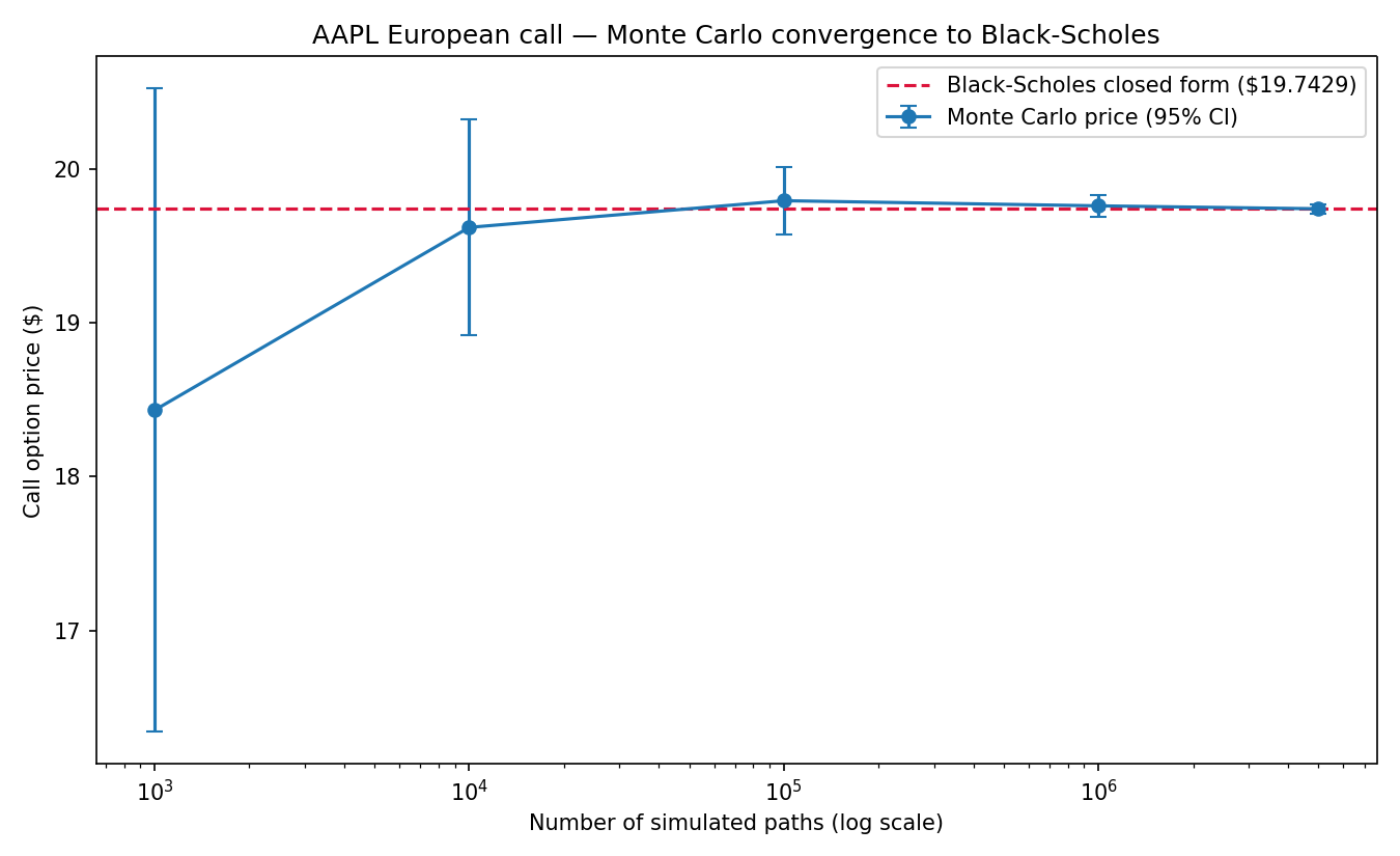
The error shrinks from -$1.32 at 1,000 paths to -$0.002 at 5,000,000 paths — a real, measured convergence, not a plot manufactured to look convincing. This is the actual claim the project makes, and it's checked, not asserted: the repo's test suite verifies the closed-form price falls inside the Monte Carlo estimate's own 99.7% confidence interval (3 standard errors), which is a real statistical check rather than a fixed tolerance picked to make a test pass.

Step 5 — Confirm variance reduction is real, not decorative

def test_antithetic_variates_reduce_standard_error():
    with_antithetic = monte_carlo_price(..., antithetic=True)
    without_antithetic = monte_carlo_price(..., antithetic=False)
    assert with_antithetic["std_error"] < without_antithetic["std_error"]

It would be easy to add antithetic variates to a pricer and never verify they're actually reducing variance — this test exists specifically so that claim is checked on every run, at the same path count, same seed, same everything except the technique itself.

Step 6 — Re-run days later, against AAPL's real price on a different day

Same code, same repo, run fresh from git clone on 2026-09-21 instead of 2026-09-17 — AAPL's real spot price and realized volatility had both moved since the original run:

Spot (S0): $336.13
Realized annualized vol (sigma), 250 trading days: 0.2497
Black-Scholes closed-form call price: $19.7429

  n_paths=    1,000  MC price=$18.4324  std_error=±$1.0654  error_vs_BS=$-1.3105
  n_paths=   10,000  MC price=$19.6198  std_error=±$0.3568  error_vs_BS=$-0.1231
  n_paths=  100,000  MC price=$19.7930  std_error=±$0.1129  error_vs_BS=$+0.0501
  n_paths=1,000,000  MC price=$19.7597  std_error=±$0.0356  error_vs_BS=$+0.0168
  n_paths=5,000,000  MC price=$19.7405  std_error=±$0.0159  error_vs_BS=$-0.0024

The same convergence shape as the original run, against different real inputs — confirming the result wasn't a coincidence of one specific day's AAPL price, and generating the exact plot the pricer produces on every run, unedited:

Monte Carlo call price converging to the Black-Scholes closed form as path count increases from 1,000 to 5,000,000, with 95% confidence interval error bars shrinking accordingly

Closing Thoughts

What real market data and a real closed-form check add here, that a from-scratch toy example wouldn't: an actual measured convergence curve against AAPL's actual volatility, not a synthetic example tuned to converge quickly; and a test suite that checks statistical claims (convergence-within-CI, variance actually reduced) instead of asserting them in a README. The honest limitations — realized vs. implied volatility, European-only, the GBM assumption both this simulation and Black-Scholes share — are stated directly rather than smoothed over, the same discipline used throughout this portfolio's other numerical and infrastructure work.

GitHub Repository: monte-carlo-option-pricer — the pricer, the Black-Scholes reference, the real-data fetch, and the five-test suite this article's convergence numbers came from.

Reviewed against AAPL market data as of 2026-09-17.

Python · Quantitative Finance · Monte Carlo Simulation · NumPy · SciPy